Saturday, May 25, 2019

Adding groupings to TopoJSON files

GeoJSON is a structured format for encoding a variety of geographic data structures like land topology, governmental boundaries, etc. It has structures for points, lines, polygons, and discontiguous collections of all of them. GeoJSON has been in use since the late 2000s.

TopoJSON is a more recent extension to GeoJSON, which brought a key innovation: when encoding the boundary between two regions, both regions contain a representation of that boundary. Using TopoJSON frequently results in much smaller files by separating out the definition of arcs from the collections of those arcs, allowing adjacent regions to both reference the same data describing the border between them. It also adds delta-encoding where points are encoded as a delta from the previous point, which tends to result in smaller numbers for dense topographical areas. TopoJSON was added as part of D3.js, an extremely popular 3d visualization JavaScript library, and has thus spread rapidly.

Today's topic is creation of customized TopoJSON files for various purposes. Mike Bostock, one of the creators of D3, wrote a series of articles about command line tools available for working with cartographic data. I wanted to develop a visualization of climate model results for regions of the world like Latin America or the Middle East and Africa, and found these articles immensely helpful in creating a TopoJSON file to support this. Part 3, which introduces TopoJSON and the CLI tools to work with it, was especially helpful.


Overview

The overall process we'll cover today is:

  1. Annotate existing geometries in a TopoJSON file with a new grouping name.
  2. Merge the annotated geometries to create new groupings.
  3. Remove the original geometries and supporting topology data.
  4. Profit!

We'll step through this series of commands:

cat world-countries.json |\
        python region_annotate.py |\
        topomerge regions=countries1 -k "d.region" |\
        topomerge countries1=countries1 -f "false" | toposimplify \
        > world_topo_regions.json


(Step 1) Annotate existing regions: region_annotate.py

We start from world-countries.json provided by David Eldersveld under an MIT license. The file defines geometry for each country by name and country code:

"countries1": {
    "type": "GeometryCollection",
    "geometries": [
        {
            "arcs": [...etc...
            ],
            "type": "MultiPolygon",
            "properties": {
                "name": "Argentina",
                "Alpha-2": "AR"
            },
            "id": "ARG"
        },

In Python, we create a tool with a mapping table of country names to the regions we want to define:

region_mapping = {
    "Albania": "Eastern Europe",
    "Algeria": "Middle East and Africa",
    "Argentina": "Latin America",

We read in the JSON, iterate over each country, and add a field for the region it is supposed to be in:

d = json.load(sys.stdin)
for country in d['objects']['countries1']['geometries']:
    name = country['properties']['name']
    region = region_mapping[name]
    country['region'] = region

json.dump(obj=d, fp=sys.stdout, indent=4)

If one were to examine the JSON at this moment, there would be a new field:

"countries1": {
    "type": "GeometryCollection",
    "geometries": [
        {
            "arcs": [...etc...
            ],
            "type": "MultiPolygon",
            "properties": {
                "name": "Argentina",
                "Alpha-2": "AR"
            },
            "id": "ARG",
            "region": "Latin America"
        },


(Step 2) Merge annotated regions: topomerge

topomerge is part of the topojson-client package of tools, and exists to manipulate geometries in TopoJSON files. We invoke TopoJSON to create new geometries using the field we just added.

topomerge regions=countries1 -k "d.region"

The "regions=countries1" argument means to use the source object "countries1" and to target a new "regions" object. The -k argument defines a key to use in creating the target objects, where d is the name of each source object being examined. We're tell it to use the 'region' field we added in step 1.

If we were to examine the JSON at this moment, the original "countries1" collection of objects would be present as well as a new "regions" collection of objects.

"objects": {
    "countries1": {
        "type": "GeometryCollection",
        "geometries": [
            {
                "arcs": [...etc...
                ],
                "type": "MultiPolygon",
                "properties": {
                    "name": "Argentina",
                    "Alpha-2": "AR"
                },
                "id": "ARG",
                "region": "Latin America"
            },
        ...etc, etc...
    "regions": {
        "type": "GeometryCollection",
        "geometries": [
            {
                "type": "MultiPolygon",
                "arcs": [...etc...
                ],
                "id": "Latin America"
            },


(Step 3) Remove original regions

As we don't use the individual countries in this application, only regions, we can make the file smaller and the UI more responsive by removing the unneeded geometries. We use topomerge to remove the "countries1" objects:

topomerge countries1=countries1 -f "false"

As before, the "countries1=countries1" argument means to use the source object "countries1", and to target the same "countries1" object. We're overwriting it. The -f argument is a filter, which takes a limited JavaScript syntax to examine each object to determine whether to keep it. In our case we're removing all of the objects unconditionally, so we pass in false.

If we were to examine the JSON at this moment, we would see an empty "countries1" collection followed by the "regions" collection we created earlier.

"objects": {
    "countries1": {
        "type": "GeometryCollection",
        "geometries": []
    },
    "regions": {
        "type": "GeometryCollection",
        "geometries": [
            {
                "type": "MultiPolygon",
                "arcs": [...etc...
                ],
                "id": "Latin America"
            },

However we're not quite done, as the arcs which define the geometry between all of those countries are still in the file, though not referenced by any object. We use toposimplify, part of the topojson-simplify package of tools, to remove the unreferenced arcs.

topomerge countries1=countries1 -f "false" | toposimplify


(Step 4) Profit!

That's it. We have a new TopoJSON file defining our regions. Rendered to PNG:

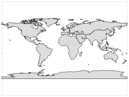
The JSON file viewed using github's gist viewer requires a bit of explanation: the country boundaries seen here are being rendered by github from OpenStreetMap data. The country boundaries are not present in the JSON file we created, only the regional boundaries as seen in the PNG file.

Tuesday, May 7, 2019

ipyvolume Frizzle Charts

ipyvolume is an extension for Jupyter notebooks which handles 3D charts and objects. There are several built-in chart types including 3D scatter plots, but those tend to work best for a single large collection of datapoints which span the whole 3D space. Trying to use a scatter plot to chart multiple (though related) series of data didn't work very well, the dots all tended to blend together into a big flock of dots.

Instead, we'll go over a custom chart implemented using a continuous visual element for the series, rather than a discrete dot per datapoint, by creating the requisite triangles and textures. As it uses strips of polygons following a path, we refer to it as a Frizzle Chart. Jumping to the punchline first:

The chart is generated from a Pandas DataFrame, where each column is turned into one of the frizzle strips. Walking through the code which builds the chart:

def get_frizzle_chart(df, ylabel, size=None, key=None):
    """Returns a 3D Frizz chart, one frizzle strip per column in the dataframe.

       Arguments:
         df: the DataFrame to graph.
         ylabel: text label to place on the Y axis.
         size: in integer pixels

       Returns:
         an ipywidget
    """
    (width, height) = (size, size) if size is not None else (500, 500)


We start by calling figure(), to create a new container to hold a chart. ipyvolume follows a pattern established by matplotlib, wherein commands are executed in an immediate mode and implicitly join a container which holds all such commands, as opposed to explicitly creating a chart object and calling methods on that object. We also create a list of colors to use for each frizzle strip.

    ipv.figure(width=width, height=height, key=key, controls=True)
    color = [(161,222,240), (56,116,114), (16,237,220), (28,69,133), (238,128,254),
            (180,39,183), (92,130,210), (22,66,205), (228,204,241), (138,68,136),
            (134,202,98), (35,137,16), (68,242,112), (106,127,47), (237,212,94),
            (103,61,23), (251,120,16), (180,39,32), (253,108,160), (184,114,90)]


We create strips of triangles, one for each column in the DataFrame. Each data point in the dataframe determines the Y-axis height of the vertices for the triangle at that point. The row index of the dataframe becomes the X-axis position. The columns turn into the Z-axis, one after another.

    # Draw a strip of triangles for each region, tracing the dataframe values
    for (z, region) in enumerate(df.columns):
        years = list(df.index)
        nyears = len(years)
        year = years.pop(0)
        X = [year, year]
        y = df.loc[year, region]
        Y = [y, y]
        Z = [float(z), float(z) + 1.0]


In graphics programming, [U, V] coordinates are offsets within a texture map. We are specifying that [X, Y, Z] in the 3D space corresponds to [U, V] in the texture. When applying a texture to the frizzle strips it will interpolate between the points where we've specified [U, V].

        U = [0.0, 0.0]
        V = [0.0, 1.0]
        triangles = []
        offset = 2
        for (idx, year) in enumerate(years, 1):
            X.extend([year, year])
            y = df.loc[year, region]
            Y.extend([y, y * 0.97])
            Z.extend([float(z), float(z) + 1.0])
            u = float(idx) / nyears
            U.extend([u, u])
            V.extend([0.0, 1.0])
            triangles.extend([[offset-2, offset-1, offset+1], [offset-2, offset, offset+1]])
            offset += 2


ipyvolume does not have a way to provide descriptive tick labels on the axes. In our case, the Z axis represents different regions of the world like "OECD90" and "Latin America," but the axis will be labelled with with the numbers zero through nine. We use the Python Imaging Library to create a texture to be mapped to each frizzle strip, giving the name of the column from the original DataFrame.

        img = PIL.Image.new(mode='RGB', size=(1000, 100), color=color[z])
        draw = PIL.ImageDraw.Draw(img)
        font = PIL.ImageFont.truetype(os.path.join('data', 'fonts', 'Roboto-Medium.ttf'), 90)
        draw.text(xy=(100, 0), text=region, fill=(255,0,0), font=font)
        ipv.pylab.plot_trisurf(np.array(X), np.array(Y), np.array(Z), triangles=triangles,
                u=U, v=V, texture=img.transpose(PIL.Image.FLIP_TOP_BOTTOM))


We set up labels for the axes and position the camera to view the completed scene. We position the camera twice to work around what appears to be a bug: the tick marks on each axis initially appear all bunched up together at the middle, and only move to their proper locations the first time the viewport is changed.

    ipv.style.box_on()
    ipv.pylab.xlabel('Year')
    first_year = df.index[0]
    last_year = df.index[-1]
    ipv.pylab.xlim(first_year - 2, last_year + 2)
    ipv.pylab.ylabel(ylabel)
    ipv.pylab.zlabel('Region')
    nregions = len(df.columns)
    ipv.pylab.zlim(-0.5, nregions + 0.5)
    ipv.pylab.view(10.0, 10.0, 3.0)
    ipv.pylab.view(-165.0, 80.0, 2.2)


Finally, we return the widget containing the frizzle graph. gcc() is "get current container," which was allocated when we called figure() at the top of the routine.

    return ipv.gcc()

For convenience, the complete routine without commentary is reproduced at the bottom of the post.


For reference, this is the DataFrame which generated the Frizzle Chart shown at the top of the post.

Year World OECD90 Eastern Europe Asia (Sans Japan) Middle East and Africa Latin America China India EU USA
2014 22548.3 9630.9 2021.8 8068.1 1750.3 1681.6 5262.8 1324.9 3379.6 4226.1
2015 24255.9 9686.1 2046.1 8517.3 1813.4 1729.4 5577.5 1407.8 3402.9 4238.2
2016 25118.0 9726.6 2070.4 8971.8 1887.4 1782.4 5868.3 1508.6 3423.0 4238.1
2017 25980.0 9770.9 2095.8 9419.6 1964.8 1838.0 6148.2 1613.2 3443.2 4240.9
2018 26841.8 9818.8 2122.1 9861.1 2045.6 1896.1 6417.4 1721.5 3463.3 4246.4
2019 27703.5 9870.2 2149.3 10296.7 2130.0 1956.8 6676.3 1833.5 3483.5 4254.5
2020 28565.2 9925.0 2177.4 10726.8 2218.1 2019.9 6925.0 1949.2 3503.9 4265.2
2021 29426.8 9983.0 2206.3 11151.8 2310.0 2085.4 7164.0 2068.5 3524.5 4278.2
2022 30288.3 10044.2 2235.9 11572.1 2405.8 2153.3 7393.5 2191.4 3545.3 4293.6
2023 31149.9 10108.3 2266.3 11988.2 2505.7 2223.6 7613.7 2317.8 3566.4 4311.3
2024 32011.6 10175.3 2297.3 12400.3 2609.7 2296.1 7825.0 2447.7 3587.9 4331.0
2025 32873.3 10245.0 2329.0 12808.9 2718.0 2370.9 8027.6 2581.1 3609.8 4352.9
2026 33735.1 10317.4 2361.2 13214.4 2830.7 2447.9 8221.8 2717.8 3632.1 4376.7
2027 34597.1 10392.2 2393.9 13617.2 2947.8 2527.1 8407.9 2858.0 3655.0 4402.3
2028 35459.2 10469.4 2427.2 14017.7 3069.7 2608.4 8586.1 3001.4 3678.5 4429.7
2029 36321.6 10548.8 2460.8 14416.3 3196.2 2691.7 8756.8 3148.1 3702.6 4458.8
2030 37184.1 10630.4 2494.9 14813.4 3327.6 2777.1 8920.3 3298.0 3727.3 4489.4
2031 38047.0 10713.9 2529.2 15209.3 3463.9 2864.5 9076.7 3451.2 3752.9 4521.5
2032 38910.2 10799.2 2563.9 15604.5 3605.4 2953.9 9226.4 3607.4 3779.2 4555.0
2033 39773.7 10886.3 2598.8 15999.4 3752.0 3045.2 9369.7 3766.8 3806.4 4589.8
2034 40637.5 10975.0 2633.9 16394.4 3903.9 3138.3 9506.9 3929.3 3834.5 4625.8
2035 41501.8 11065.1 2669.1 16789.9 4061.3 3233.3 9638.2 4094.7 3863.5 4662.9
2036 42366.5 11156.6 2704.4 17186.2 4224.2 3330.1 9763.9 4263.1 3893.6 4700.9
2037 43231.6 11249.3 2739.8 17583.8 4392.8 3428.6 9884.3 4434.5 3924.8 4739.9
2038 44097.3 11343.0 2775.2 17983.0 4567.1 3528.8 9999.7 4608.8 3957.1 4779.7
2039 44963.4 11437.8 2810.5 18384.3 4747.4 3630.7 10110.4 4785.9 3990.6 4820.2
2040 45830.2 11533.3 2845.7 18788.1 4933.6 3734.2 10216.6 4965.8 4025.3 4861.3
2041 46697.5 11629.6 2880.8 19194.7 5125.9 3839.2 10318.6 5148.5 4061.3 4903.0
2042 47565.5 11726.5 2915.6 19604.5 5324.5 3945.9 10416.7 5333.9 4098.7 4945.0
2043 48434.1 11823.8 2950.3 20018.0 5529.4 4053.9 10511.2 5521.9 4137.4 4987.5
2044 49303.3 11921.4 2984.6 20435.6 5740.8 4163.5 10602.4 5712.6 4177.7 5030.1
2045 50173.4 12019.2 3018.7 20857.6 5958.8 4274.5 10690.5 5905.9 4219.4 5072.9
2046 51044.1 12117.1 3052.3 21284.5 6183.5 4386.8 10775.9 6101.8 4262.8 5115.7
2047 51915.6 12215.0 3085.5 21716.6 6414.9 4500.4 10858.8 6300.1 4307.7 5158.5
2048 52788.0 12312.6 3118.2 22154.3 6653.3 4615.3 10939.4 6501.0 4354.4 5201.2
2049 53661.2 12410.0 3150.4 22598.1 6898.8 4731.5 11018.2 6704.2 4402.8 5243.6
2050 54535.3 12506.9 3182.0 23048.3 7151.4 4848.9 11095.2 6909.8 4452.9 5285.6
2051 55410.3 12603.3 3213.0 23505.3 7411.2 4967.4 11171.0 7117.8 4505.0 5327.3
2052 56286.2 12698.9 3243.3 23969.5 7678.5 5087.0 11245.6 7328.0 4558.9 5368.4
2053 57163.1 12793.8 3272.9 24441.4 7953.3 5207.7 11319.4 7540.5 4614.8 5408.9
2054 58041.0 12887.7 3301.8 24921.3 8235.6 5329.4 11392.8 7755.2 4672.7 5448.7
2055 58920.0 12980.5 3329.8 25409.6 8525.7 5452.2 11465.8 7972.1 4732.6 5487.7
2056 59800.0 13072.1 3357.0 25906.8 8823.7 5575.8 11539.0 8191.1 4794.7 5525.8
2057 60681.1 13162.5 3383.2 26413.1 9129.6 5700.4 11612.4 8412.1 4859.0 5562.8
2058 61563.4 13251.3 3408.5 26929.1 9443.6 5825.8 11686.5 8635.3 4925.5 5598.8
2059 62446.8 13338.6 3432.8 27455.1 9765.8 5952.0 11761.4 8860.4 4994.3 5633.6
2060 63331.4 13424.2 3456.0 27991.4 10096.3 6079.1 11837.5 9087.4 5065.5 5667.1


The code without commentary:

def get_frizzle_chart(df, ylabel, size=None, key=None):
    """Returns a 3D Frizz chart, one frizzle strip per column in the dataframe.

       Arguments:
         df: the DataFrame to graph.
         ylabel: text label to place on the Y axis.
         size: in integer pixels

       Returns:
         an ipywidget
    """
    (width, height) = (size, size) if size is not None else (500, 500)
    ipv.figure(width=width, height=height, key=key, controls=True)
    color = [(161,222,240), (56,116,114), (16,237,220), (28,69,133), (238,128,254),
            (180,39,183), (92,130,210), (22,66,205), (228,204,241), (138,68,136),
            (134,202,98), (35,137,16), (68,242,112), (106,127,47), (237,212,94),
            (103,61,23), (251,120,16), (180,39,32), (253,108,160), (184,114,90)]

    # Draw a strip of triangles for each region, tracing the dataframe values
    for (z, region) in enumerate(df.columns):
        years = list(df.index)
        nyears = len(years)
        year = years.pop(0)
        X = [year, year]
        y = df.loc[year, region]
        Y = [y, y]
        Z = [float(z), float(z) + 1.0]
        U = [0.0, 0.0]
        V = [0.0, 1.0]
        triangles = []
        offset = 2
        for (idx, year) in enumerate(years, 1):
            X.extend([year, year])
            y = df.loc[year, region]
            Y.extend([y, y * 0.97])
            Z.extend([float(z), float(z) + 1.0])
            u = float(idx) / nyears
            U.extend([u, u])
            V.extend([0.0, 1.0])
            triangles.extend([[offset-2, offset-1, offset+1], [offset-2, offset, offset+1]])
            offset += 2
        img = PIL.Image.new(mode='RGB', size=(1000, 100), color=color[z])
        draw = PIL.ImageDraw.Draw(img)
        font = PIL.ImageFont.truetype(os.path.join('data', 'fonts', 'Roboto-Medium.ttf'), 90)
        draw.text(xy=(100, 0), text=region, fill=(255,0,0), font=font)
        ipv.pylab.plot_trisurf(np.array(X), np.array(Y), np.array(Z), triangles=triangles,
                u=U, v=V, texture=img.transpose(PIL.Image.FLIP_TOP_BOTTOM))

    ipv.style.box_on()
    ipv.pylab.xlabel('Year')
    first_year = df.index[0]
    last_year = df.index[-1]
    ipv.pylab.xlim(first_year - 2, last_year + 2)
    ipv.pylab.ylabel(ylabel)
    ipv.pylab.zlabel('Region')
    nregions = len(df.columns)
    ipv.pylab.zlim(-0.5, nregions + 0.5)
    ipv.pylab.view(10.0, 10.0, 3.0)
    ipv.pylab.view(-165.0, 80.0, 2.2)
    return ipv.gcc()