In the previous post about charting options for Jupyter Notebooks, the container to run the Notebook had to include a number of extensions for JupyterLab to enable the various charting packages to work. JupyterLab, the next major version of Juypter Notebooks, locks down JavaScript within the Notebook web environment and requires extensions to facilitate it for each package.
jupyter labextension install jupyter-matplotlib
jupyter labextension install bqplot
jupyter labextension install jupyterlab_bokeh
jupyter labextension install beakerx-jupyterlab
jupyter labextension install @pyviz/jupyterlab_pyviz
jupyter labextension install @jupyterlab/plotly-extension
All except one charting package required an extension, that is. The one which doesn't is Altair, which works not by generating JavaScript but by generating a Vega-Lite description of the desired chart. Vega is a visualization grammar, a declarative language for describing visualization. For example, consider the first few lines of a bar chart example from the Vega site:
{
  "$schema": "https://vega.github.io/schema/vega/v5.json",
  "width": 400,
  "height": 200,
  "padding": 5,

  "data": [
    {
      "name": "table",
      "values": [
        {"category": "A", "amount": 28},
        {"category": "B", "amount": 55},
        {"category": "C", "amount": 43},
        {"category": "D", "amount": 91},
        {"category": "E", "amount": 81},
        {"category": "F", "amount": 53},
        {"category": "G", "amount": 19},
        {"category": "H", "amount": 87}
      ]
    }
  ],
JupyterLab includes a renderer for Vega-Lite and Vega. A Vega description can be passed to JupyterLab's display() routine, and will render graphically in the Notebook. This means we can write code within the Notebook to generate a Vega description, and then render it, without requiring any extension to be installed.
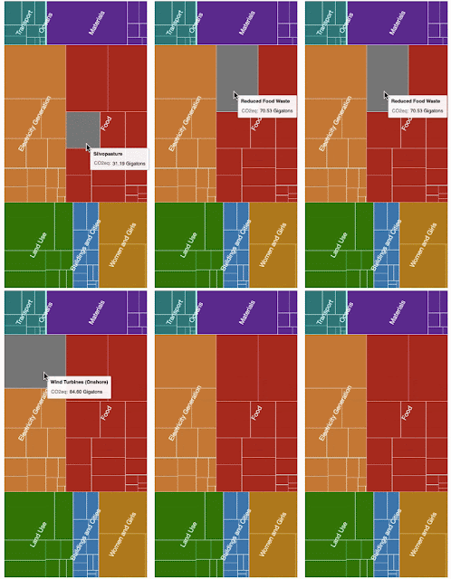
As one example: consider an interactive treemap. None of the charting packages investigated earlier had a treemap implementation which I really liked, but the Vega grammar supports one. Using Python code running within the Notebook, we can generate one:
# Vega treemap documentation: https://vega.github.io/vega/examples/treemap/
  return {
      "$schema": "https://vega.github.io/schema/vega/v4.json",
      "width": width,
      "height": height,
      "padding": 2.5,
      "autosize": "none",

      "signals": [
        {
          "name": "layout", "value": "squarify",
        },
        {
          "name": "aspectRatio", "value": 1.6,
        }
      ],

      "data": [
        {
          "name": "drawdown",
          "values": list(elements.values()),
          "transform": [
            {
              "type": "stratify",
              "key": "id",
              "parentKey": "parent"
            },
            {
              "type": "treemap",
              "field": "size",
              "sort": {"field": "value"},
              "round": True,
              "method": {"signal": "layout"},
              "ratio": {"signal": "aspectRatio"},
              "size": [{"signal": "width"}, {"signal": "height"}]
            }
          ]
        },
        {
          "name": "nodes",
          "source": "drawdown",
          "transform": [{ "type": "filter", "expr": "datum.children" }]
        },
        {
          "name": "leaves",
          "source": "drawdown",
          "transform": [{ "type": "filter", "expr": "!datum.children" }]
        }
      ],
      "scales": [
        {
          "name": "color",
          "type": "ordinal",
          "domain": list(sector_colormap.keys()),
          "range": list(sector_colormap.values())
        },
      ],

      "marks": [
        {
          "type": "rect",
          "from": {"data": "nodes"},
          "interactive": False,
          "encode": {
            "enter": {
              "fill": {"scale": "color", "field": "name"}
            },
            "update": {
              "x": {"field": "x0"},
              "y": {"field": "y0"},
              "x2": {"field": "x1"},
              "y2": {"field": "y1"}
            }
          }
        },
        {
          "type": "rect",
          "from": {"data": "leaves"},
          "encode": {
            "enter": {
              "stroke": {"value": "#fff"},
              "tooltip": {
                "signal": "{title: datum.name, 'CO2eq': datum.size + ' Gigatons'}"}
            },
            "update": {
              "x": {"field": "x0"},
              "y": {"field": "y0"},
              "x2": {"field": "x1"},
              "y2": {"field": "y1"},
              "fill": {"value": "transparent"}
            },
            "hover": {
              "fill": {"value": "gray"}
            }
          }
        },
        {
          "type": "text",
          "from": {"data": "nodes"},
          "interactive": False,
          "encode": {
            "enter": {
              "font": {"value": "Helvetica Neue, Arial"},
              "align": {"value": "center"},
              "baseline": {"value": "middle"},
              "fill": {"value": "#fff"},
              "text": {"field": "name"},
              "fontSize": {"value": 18},
              "fillOpacity": {"value": 1.0},
              "angle": {"value": -62.0}
            },
            "update": {
              "x": {"signal": "0.5 * (datum.x0 + datum.x1)"},
              "y": {"signal": "0.5 * (datum.y0 + datum.y1)"}
            }
          }
        }
      ]
    }
The text string is passed to JupyterLab's display() method, annotated with the MIME-type:
display(
   {'application/vnd.vega.v4+json': solution_treemap(width=400, height=800)},
   raw=True)
The resulting treemap looks like this:
The notebook can be run for keepsies using mybinder.org, which creates a container to run user code. Clicking on the button below will open Jupyter in a new browser window, albeit after a perhaps lengthy pause while initializing a container to run it.

For those who have not used Jupyter before: each numbered block of code in the Notebook is a cell, and can be run using the right-pointing triangle button at the top. When the Notebook is first opened there will likely be no graphs displayed. Clicking the run button in each cell will run it and display the treemap.


